
This tutorial is for readers who already know basic classes in Python and want a clean, iterative BST with insert, search, delete, and traversals—without a global root variable. You will see how a BST differs from an ordinary binary tree, how the three deletion cases work, and how to reason about complexity and duplicates. For general tree terminology and traversals, start with Python tree data structure; to time search on large trees, see measure execution time.
The runnable example at the end uses only the Python standard library, includes assert lines as self-checks, and was executed locally with the version shown below.
Tested on: Python 3.13.3; kernel 6.14.0-37-generic.
What is a binary search tree?
A binary search tree (BST) is a binary tree where each node holds a comparable key (often an integer), and the keys are arranged so that lookup by comparison is efficient. At every node, the left subtree contains only smaller keys and the right subtree contains keys that are greater—or greater-or-equal if you adopt a duplicate policy (covered later). For more background on trees in general, see the Python tree data structure guide.
Binary tree vs binary search tree
A binary tree only caps each node at two children; there is no ordering constraint, so search might require scanning the whole tree. A BST adds the ordering invariant so you can decide at each step whether to go left or right, like binary search on a sorted array—but laid out as a linked structure.
Binary search tree rules
For every node n with key k: all keys in n.left are < k (for a strict-left duplicate policy), and all keys in n.right are > k or >= k depending on how you treat duplicates. The empty tree has no nodes; a single-node tree is a valid BST. Inorder traversal (left, node, right) visits keys in sorted order when keys are unique and the strict < / > rule holds.
Create a BST node and tree structure in Python
A node stores a key and references to left and right children, which may be None. A small BST class holds the root pointer and keeps all operations in one place instead of using module-level globals.
from __future__ import annotations

from typing import Optional


class Node:
    def __init__(self, key: int) -> None:
        self.key = key
        self.left: Optional[Node] = None
        self.right: Optional[Node] = None


class BST:
    def __init__(self) -> None:
        self.root: Optional[Node] = None
Insert a node in binary search tree
Start at root. If the tree is empty, the new node becomes the root. Otherwise walk with a pointer: if the new key is less than the current key, go left; if there is no left child, attach the new node and stop. If the key is greater (or equal under your duplicate rule), do the symmetric step on the right. This loop is iterative—no recursion stack—and runs in O(h) time for height h.
def insert(self, key: int) -> None:
        if self.root is None:
            self.root = Node(key)
            return
        cur = self.root
        while True:
            if key < cur.key:
                if cur.left is None:
                    cur.left = Node(key)
                    return
                cur = cur.left
            else:
                if cur.right is None:
                    cur.right = Node(key)
                    return
                cur = cur.right
Search a value in binary search tree
Search mirrors insert: walk from the root, comparing the target to each node’s key until you find a match or fall off the tree (None). Return a boolean or the node reference depending on your API.
def search(self, key: int) -> bool:
        cur = self.root
        while cur is not None:
            if key == cur.key:
                return True
            if key < cur.key:
                cur = cur.left
            else:
                cur = cur.right
        return False
Traverse binary search tree
Traversal is still O(n) because every node is visited once, but the order of visits changes what the sequence means. For a valid BST with unique keys, inorder output is sorted ascending—useful for debugging.
Inorder traversal
Visit left subtree, current node, then right subtree. Recursive form is short; an iterative version uses an explicit stack (not shown here) if you fear deep recursion on skewed trees.
def inorder_keys(self) -> list[int]:
        out: list[int] = []

        def walk(node: Optional[Node]) -> None:
            if node is None:
                return
            walk(node.left)
            out.append(node.key)
            walk(node.right)

        walk(self.root)
        return out
Preorder and postorder traversal
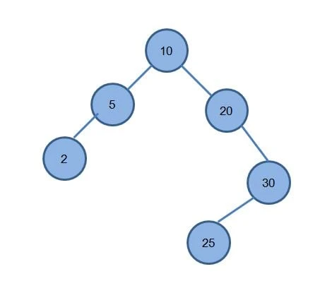
Preorder (node, left, right) is handy for copying or serializing a tree shape. Postorder (left, right, node) is natural when you must delete children before a parent in other tree problems. For a BST built from 10, 5, 20, 30, 25, 2, preorder and postorder lists differ from inorder; the full program below prints them after deletes.
def preorder_keys(self) -> list[int]:
        out: list[int] = []

        def walk(node: Optional[Node]) -> None:
            if node is None:
                return
            out.append(node.key)
            walk(node.left)
            walk(node.right)

        walk(self.root)
        return out

    def postorder_keys(self) -> list[int]:
        out: list[int] = []

        def walk(node: Optional[Node]) -> None:
            if node is None:
                return
            walk(node.left)
            walk(node.right)
            out.append(node.key)

        walk(self.root)
        return out
Delete a node from binary search tree
Deletion must preserve the BST invariant. First locate the node (and conceptually its parent); then apply one of three structural cases. All cases are O(h) when implemented iteratively or with tail recursion on the path.
Delete a leaf node
If the target has no children, remove the link from its parent (or clear root if it is the only node).
Example: after building the tree from 10, 5, 20, 30, 25, 2, node 25 is a leaf under 30.
10
       /  \
      5    20
     /      \
    2       30
           /
          25   <- leaf
Deleting 25 clears 30.left. The rest of the structure is unchanged.
Delete a node with one child
Splice the child upward in place of the deleted node: the parent’s left or right pointer now references that single subtree, which keeps ordering because every key in that subtree was already on the correct side of the parent chain.
Mini-example on its own:
20
   /
  10
   \
   15
Deleting 10 leaves only 15 in that subtree, so 20.left should point to 15. There is no need to touch 15’s children because 10 had exactly one child.
Delete a node with two children
You cannot simply remove the node without a replacement strategy. The usual approach is to copy the key of the inorder successor—the smallest key in the right subtree—into the current node, then delete the successor node from the right subtree. That successor sits at the leftmost position and has at most one child, so deletion reduces to an easier case.
On the sample tree above, deleting the root 10 copies the successor key 20 into the root position, then removes the old 20 node (which had only a right child 30). The keys stay organized; inorder_keys becomes [2, 5, 20, 30].
def _min_key_node(self, node: Node) -> Node:
        while node.left is not None:
            node = node.left
        return node

    def delete(self, key: int) -> bool:
        self.root, found = self._delete_node(self.root, key)
        return found

    def _delete_node(self, node: Optional[Node], key: int) -> tuple[Optional[Node], bool]:
        if node is None:
            return None, False
        if key < node.key:
            node.left, found = self._delete_node(node.left, key)
            return node, found
        if key > node.key:
            node.right, found = self._delete_node(node.right, key)
            return node, found
        found = True
        if node.left is None:
            return node.right, found
        if node.right is None:
            return node.left, found
        succ = self._min_key_node(node.right)
        node.key = succ.key
        node.right, _ = self._delete_node(node.right, succ.key)
        return node, found
Handle duplicate values in BST
A strict “left < parent < right” rule leaves no room for equal keys unless you relax one comparison to <= or >=, or you refuse duplicates in insert. This article’s insert sends ties to the right (if key < cur.key else go right). Use the same rule in search and delete so behavior stays predictable. The runnable listing later also builds a small tree with repeated keys and prints its inorder keys so you can see one concrete outcome.
Time complexity of binary search tree operations
Insert, search, and delete walk from the root along one path, so each costs O(h) time and O(1) extra space for the iterative insert/search shown here (recursive delete uses O(h) stack). With random-ish insert order, h is often Θ(log n); if keys arrive sorted and you never rebalance, the tree can become a chain of height n − 1 and those same operations become O(n). Self-balancing trees or a hash-based map like Python’s dict avoid that worst case for map workloads.
Recursive vs iterative BST implementation
Recursive code matches the mathematical definition of the tree (mirror the three cases in the function for node). It is easy to read but can hit recursion limits on very deep skewed trees. Iterative code with explicit while loops (as in insert and search above) avoids that stack growth for those operations; delete is often still written recursively on the path, as in _delete_node, which is depth-bounded by h. The program below uses iteration for insert and search and recursion for delete and traversals—you can rewrite traversals with an explicit stack if you need to.
The listing is one file you can save and run with python yourfile.py; it matches the fragments in earlier sections when pasted into a single class body.
from __future__ import annotations

from typing import Optional


class Node:
    def __init__(self, key: int) -> None:
        self.key = key
        self.left: Optional[Node] = None
        self.right: Optional[Node] = None


class BST:
    def __init__(self) -> None:
        self.root: Optional[Node] = None

    def insert(self, key: int) -> None:
        if self.root is None:
            self.root = Node(key)
            return
        cur = self.root
        while True:
            if key < cur.key:
                if cur.left is None:
                    cur.left = Node(key)
                    return
                cur = cur.left
            else:
                if cur.right is None:
                    cur.right = Node(key)
                    return
                cur = cur.right

    def search(self, key: int) -> bool:
        cur = self.root
        while cur is not None:
            if key == cur.key:
                return True
            if key < cur.key:
                cur = cur.left
            else:
                cur = cur.right
        return False

    def _min_key_node(self, node: Node) -> Node:
        while node.left is not None:
            node = node.left
        return node

    def delete(self, key: int) -> bool:
        self.root, found = self._delete_node(self.root, key)
        return found

    def _delete_node(self, node: Optional[Node], key: int) -> tuple[Optional[Node], bool]:
        if node is None:
            return None, False
        if key < node.key:
            node.left, found = self._delete_node(node.left, key)
            return node, found
        if key > node.key:
            node.right, found = self._delete_node(node.right, key)
            return node, found
        found = True
        if node.left is None:
            return node.right, found
        if node.right is None:
            return node.left, found
        succ = self._min_key_node(node.right)
        node.key = succ.key
        node.right, _ = self._delete_node(node.right, succ.key)
        return node, found

    def inorder_keys(self) -> list[int]:
        out: list[int] = []

        def walk(n: Optional[Node]) -> None:
            if n is None:
                return
            walk(n.left)
            out.append(n.key)
            walk(n.right)

        walk(self.root)
        return out

    def preorder_keys(self) -> list[int]:
        out: list[int] = []

        def walk(n: Optional[Node]) -> None:
            if n is None:
                return
            out.append(n.key)
            walk(n.left)
            walk(n.right)

        walk(self.root)
        return out

    def postorder_keys(self) -> list[int]:
        out: list[int] = []

        def walk(n: Optional[Node]) -> None:
            if n is None:
                return
            walk(n.left)
            walk(n.right)
            out.append(n.key)

        walk(self.root)
        return out


if __name__ == "__main__":
    t = BST()
    for x in (10, 5, 20, 30, 25, 2):
        t.insert(x)
    print("inorder after insert:", t.inorder_keys())
    assert t.inorder_keys() == [2, 5, 10, 20, 25, 30]
    print("search 25:", t.search(25), "search 99:", t.search(99))
    assert t.search(25) and not t.search(99)
    assert t.delete(25)
    print("after delete 25:", t.inorder_keys())
    assert t.inorder_keys() == [2, 5, 10, 20, 30]
    assert t.delete(10)
    print("after delete 10:", t.inorder_keys())
    assert t.inorder_keys() == [2, 5, 20, 30]
    print("preorder:", t.preorder_keys())
    print("postorder:", t.postorder_keys())
    assert t.preorder_keys() == [20, 5, 2, 30]
    assert t.postorder_keys() == [2, 5, 30, 20]
    assert t.search(20) and not t.search(25)

    dup = BST()
    for k in (10, 10, 5, 15, 10):
        dup.insert(k)
    print("duplicates-right inorder:", dup.inorder_keys())
    assert dup.inorder_keys() == [5, 10, 10, 10, 15]

    linear = BST()
    for k in range(1, 6):
        linear.insert(k)
    print("sorted inserts inorder:", linear.inorder_keys())
    assert linear.inorder_keys() == [1, 2, 3, 4, 5]

print("all checks passed")Running it prints the insert and delete traces, preorder [20, 5, 2, 30] and postorder [2, 5, 30, 20] on the final tree, then duplicates-right inorder: [5, 10, 10, 10, 15] and sorted inserts inorder: [1, 2, 3, 4, 5], and ends with all checks passed if every assert succeeds.
Common mistakes in BST implementation
- Using a module-level
rootwith loose functions makes tests brittle and prevents multiple trees; keeprooton a class instance. - Forgetting the empty tree: handle
insertwhenrootisNoneanddeleteon an empty structure before walking. - Wrong parent updates on delete: when splicing a child, update the correct side (
leftvsright) of the parent along the search path. - Two-child delete without successor logic: copying from the wrong side or failing to delete the successor leaves duplicate keys or breaks order.
- Mixing duplicate policies: using
<=in insert but strict<in search can strand keys that should still be reachable. - Deep recursion on skewed trees: prefer iterative insert and search, or rewrite traversals with an explicit stack, instead of raising the recursion limit as a habit.
Binary search tree quick reference table
| Operation | Average time | Worst-case time | Notes |
|---|---|---|---|
| Search | O(log n) |
O(n) |
Height-limited |
| Insert | O(log n) |
O(n) |
Same walk as search |
| Delete | O(log n) |
O(n) |
Three structural cases |
| Inorder traversal | O(n) |
O(n) |
Sorted for strict BST keys |
| Space (iterative insert/search) | O(1) extra |
O(1) extra |
Aside from the tree itself |
Summary
A binary search tree keeps keys ordered so you can move left or right by comparison. This article used a Node and BST class with iterative insert and search, recursive helpers for delete and traversals, and the standard successor-based deletion for two-child nodes. Duplicates require an explicit convention, and height governs performance—sorted input without balancing yields a linked-list shape and linear-time operations. The combined listing under the section “Recursive vs iterative BST implementation” is a runnable reference you can extend (for example with rank queries or a self-balancing variant).